Asteroid Diameter Prediction Final Report
Introduction
There are over one million known asteroids in our solar system, and it is suspected that there are millions more yet to be discovered. These asteroids are irregularly shaped, rocky, and range in size from one meter to hundreds of kilometers in diameter [2]. While some of the known asteroids have measured diameters, many do not. Due to technological, financial, and time limitations, it is not possible to directly measure the diameters of many of these asteroids.
Problem Definition
The Jet Propulsion Laboratory of NASA maintains a database cataloging known asteroids and storing features including their distance from the sun, eccentricity, and more. So far, scientists have measured the diameter of approximately 16% of the total known asteroids. For our project, we will develop a machine learning based prediction system for asteroid diameters. We will utilize a cleaned version of JPL’s asteroid catalogue from Kaggle as a dataset to train and test the prediction system.
As more asteroids are discovered and cataloged, our system can be used to quickly and cost-effectively estimate their diameters. Armed with this information, scientists and policymakers can help predict the danger posed by an Earth-intercepting asteroid. It can also aid in our understanding of how the solar system formed and how bodies interact in space.
Data Collection
We used the Open Asteroid Dataset on Kaggle which provides data on over 800,000 asteroids [4]. The dataset includes 31 features, each one providing different characteristics about the asteroid. Among those features, we noticed that there were some which should not have an intrinsic relationship with the diameter of the asteroid: for example, the name of the asteroid or the number of days over which the data was collected. For this reason, we went through each feature, and checked its relevance to our problem. In the table below, you can find each feature, with its description and explanation.
| Feature | Description | Explanation |
|---|---|---|
| a | semi-major axis(au) | one half of the major axis of the elliptical orbit; also the mean distance from the Sun [12] |
| e | eccentricity | the mean distance from the Sun [12] |
| i | Inclination with respect to x-y ecliptic plane(deg) | angle between the orbit plane and the ecliptic plane [12] |
| om | Longitude of the ascending node | "point on the orbit where the object “ascends” through the ecliptic plane, passing from below it to above it [12]" |
| w | argument of perihelion | angle in the orbit plane between the ascending node and the perihelion point [12] |
| q | perihelion distance(au) | an orbit’s closest point to the Sun [12] |
| ad | aphelion distance(au) | an orbit’s farthest point to the Sun [12] |
| per_y | Orbital period(YEARS) | time it takes to make one complete revolution around the Sun in years [12] |
| data_arc | data arc-span(d) | the number of days of the orbit over which the object has been observed for |
| condition_code | Orbit condition code | how well an object's orbit is known on a logarithmic scale |
| n_obs_used | Number of observation used | number of observations used |
| H | Absolute Magnitude parameter | the luminosity of a celestial object |
| neo | Near Earth Object | has a perihelion distance less than or equal to 1.3 au [12] |
| pha | Physically Hazardous Asteroid | a minimum orbit intersection distance of 0.05 au or less and an absolute magnitude of 22.0 or less [12] |
| extent | Object bi/tri axial ellipsoid dimensions(Km) | bi/tri axial ellipsoid dimensions |
| albedo | geometric albedo | ratio of the light received by a body to the light reflected by that body [12] |
| rot_per | Rotation Period(h) | time it takes to do one revolution around axis of rotation |
| GM | Standard gravitational parameter | product of mass and gravitational constant |
| BV | Color index B-V magnitude difference | determine the color of an object using B and V filters |
| UB | Color index U-B magnitude difference | determine the color of an object using U and B filters |
| IR | Color index I-R magnitude difference | determine the color of an object using I and R filters |
| spec_B | Spectral taxonomic type(SMASSII) | more recent taxonomy based on higher-resolution spectral data |
| spec_T | Spectral taxonomic type(Tholen) | "most widely used taxonomy for asteroid classification, largely based off of albedo" |
| G | Magnitude slope parameter | "based on the opposition effect, measures the surge in brightness when the object is near opposition" |
| moid | Earth Minimum orbit Intersection Distance(au) | assess potential close approaches and collision risks |
| class | asteroid orbit class | describes the orbit of an asteroid |
| n | Mean motion(deg/d) | average angular frequency of the orbit |
| per | orbital Period(d) | time to do one cycle around the sun in years |
Our first step was to clean the data set. We did this using the Python library Pandas. Approximately 140,000 samples from the dataset include the asteroids’ diameters, while the remaining samples do not have a known diameter. We removed all data samples that had no diameter so we could use the remaining data to conduct supervised learning. To further clean the data, we removed any samples which had missing data for any of the features. As the relative proportion of missing data was low, we were not concerned with removing all samples that contained missing data. Next, we converted non-numerical features, such as text-based categorical features, like whether or not an asteroid is potentially hazardous, into numerical values. For columns containing binary classifications, we substituted in 0/1. Finally, we removed features that were not relevant to the prediction task, including metadata regarding the asteroid and the observations taken of the asteroid (features removed: _name, class, G, extent, rot_per, GM, BV, UB, IR, spec_B, and spec_T_). After cleaning the data, approximately 136,000 data samples, each with 19 features remained.
We conducted experiments with the XGBoost, ridge, lasso, and random forest regressors with the following data configurations:
- Without dimensionality reduction or data standardization, all 19 features are utilized.
- Utilize dimensionality reduction (PCA) with standardization, converting the original 19 features into three features.
- Utilizing domain expertise, running experiments on only luminosity and albedo, the two measures that are known to provide a good estimate for asteroid diameter.
For the sake of brevity, we will only discuss a subset of these experiments at length in the Results section.
In the classification experiments, we utilized two data configurations:
- Utilizing all 19 features (no dimensionality reduction).
- Utilize dimensionality reduction (PCA) without standardization (three features).
Finally, in experiments conducted with neural networks, we utilized two data configurations:
- Only utilize albedo and H (luminosity).
- Utilize albedo, H, and per_y.
We chose these columns for experimentation as they followed from domain expertise, as elaborated in [12].
Covariance Matrix
From our first set of features, we generated a covariance matrix which can be accessed through the following link: Covariance Matrix
We noticed that the feature that had the greatest covariance with diameter was data_arc. Recall that data_arc represents the number of days that data was collected over for a certain asteroid. We can deduce that this is the result of larger asteroids being easier to study or more important to researchers. However, this feature is not an intrinsic property of the asteroid. For this reason, we knew that it would not necessarily be a useful feature to predict the diameters of new asteroids. We know from [12] that albedo and H should be better at predicting diameters so we ran RandomForest on combinations of the two and here were the resulting r^2 scores.
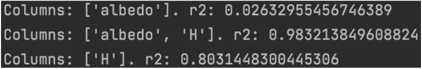
Figure 1: r^2 scores of runnning RandomForest with H and albedo.
After doing research on all of our features, we found that H and albedo should have a direct relationship with diameter. We recalculated our covariance matrix, with only three features: diameter, H, and albedo. We found H had a high negative covariance with the diameter -7.516429, motivating us to work further with that feature.
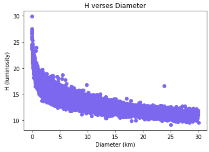
Figure 2: Scatterplot of H vs. diameter.
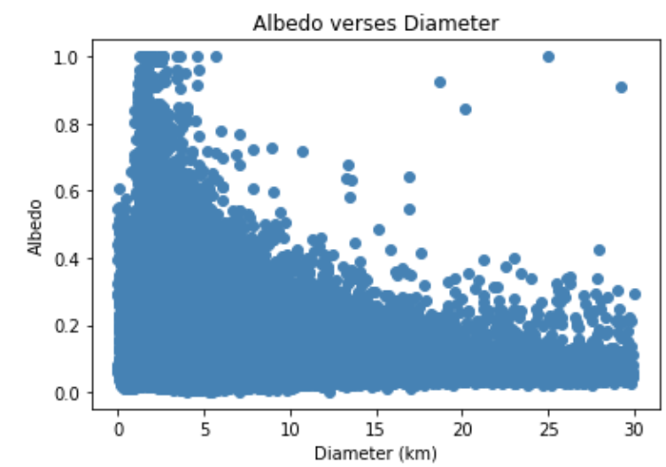
Figure 3: Scatterplot of Albedo vs. diameter.
Note: For these graphs, we only include asteroids with diameters <= 30
since the diameter increases at a much faster magnitude than either H
or albedo decreases. For reference, the largest diameter an asteroid
in our data has is 939.4 kilometers.
From the graphs, we can see that H and diameter have a strong negative relationship. In contrast, we can see the relationship between diameter and albedo is not as strong.
Feature Reduction
Using sklearn, we performed principal component analysis (PCA). We reduced our dataset from 19 features to three features with a retained variance of over 99% . The results of PCA are shown in the below figures. The different colors of the points on the graph represent the target where black represents training data, yellow represents testing data, and red represents predicted values. As is clearly visible, it is hard to distinguish between data of different colors. We note that this indicates that the dimensionality-reduced data does not display a clear trend.
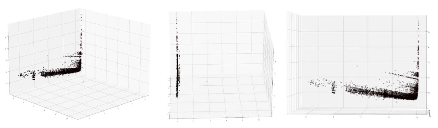
Figure 4: Result of performing PCA to reduce the dataset to 3 features.
Additionally, we also used t-SNE, which is a tool to visualize high-dimensional data while minimizing “the Kullback-Leibler divergence between the joint probabilities of the low-dimensional embedding and the high-dimensional data” [5]. We set the number of components equal to two and used an ‘auto’ learning rate with a random initialization. The results showed that despite limiting the number of columns used to be components of the most important ones, the predicted values got closer to the actual labels, but it still was not close enough to be a model we would actually consider.
The code we utilized to run t-SNE is as follows (where features are the features in our dataset):
reduced_tsne = TSNE(n_components=2, learning_rate='auto', init='random').fit_transform(features)
Finally, we also explored Locally Linear Embedding as an additional dimension reduction technique in an attempt to find a “projection of the data which preserves distances within local neighborhoods.” In short, this method compares several local iterations of PCA to find the most fitting nonlinear embedding [6]. We set the number of components equal to three. The results showed that LLE was largely unsuccessfully fully representing the model.
The code we utilized to run Locally Linear Embedding is as follows (where features are the features in our dataset):
reduced_lle = LocallyLinearEmbedding(n_components=3).fit_transform(features)
lle_x_train, lle_x_test, lle_y_train, lle_y_test = train_test_split(reduced_lle, target, test_size=0.2, random_state=28)
Standardization
Finally, before running training, we standardize the preprocessed data using a Standard Scaler, which removes the mean and scales the data to unit variance to make the data look normally distributed [7].
The code we utilized to run standardization is as follows (where features are the features in our dataset):
standardized_data = preprocessing.StandardScaler().fit(reduced_pca).transform(reduced_pca)
processed_df = pd.DataFrame(standardized_data)
Methods
Throughout our experimentation, we explored a varied set of algorithms, data configuration, and learning methods. We break each of these different scenarios out below. For all algorithms, we used k-folds cross validation with k=10 for each candidate.
Classification
Upon explaining our difficulties with training our model, a TA suggested that we attempt to use a classification model with binned diameters. We created a histogram (figure 2) to gauge the distribution of diameter sizes and created the bins outlined in figure 3. We dropped the diameter column and replaced it with a category column which held the bin that the original diameter belonged to.
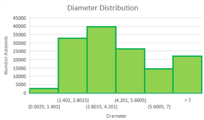
Figure 5: Diameter distribution.
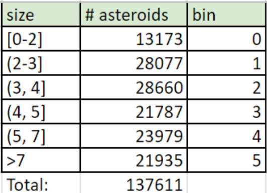
Figure 6: Diameter categories.
Due to time constraints, we were only able to investigate a limited set of options, both in terms of data configuration and learning algorithms. Specifically, we explored the Decision Tree classifier to train the data [15]. For this classifier, the code we utilized to run training is as follows (where features are the processed data from the training dataset):
clf = tree.DecisionTreeClassifier()
y_pred = cross_val_predict(clf, features, target, cv=10)
multiconf = multilabel_confusion_matrix(target, y_pred, labels=[0,1,2,3,4,5])
Regression
The bulk of our efforts focused on developing a successful regression model to predict asteroid diameters.
Ridge Regression
Utilizing our knowledge from class, we trained our data using sklearn.linear_model.Ridge which uses regularization to avoid overfitting. The goal of this method is to “minimize the residual sum of squares between the observed targets in the dataset” [8].
The code we utilized to run training including executing a grid search for hyperparameter optimization is as follows (where processed_df are the processed data):
from sklearn.linear_model import Ridge
param_grid = {
    "alpha": [0.01, 0.02, 0.03, 0.04, 0.05, 0.1, 0.2, 0.5, 1.0, 1.5, 2.0, 2.5, 5.0, 7.5, 10.0],}
clf = Ridge()
grid_search = GridSearchCV(clf, cv=10, param_grid=param_grid, scoring='neg_root_mean_squared_error', n_jobs=-1, verbose=3)
grid_search.fit(processed_df, target)
We optimized the alpha hyperparameter, utilizing a grid search with the choices 0.01, 0.02, 0.03, 0.04, 0.05, 0.1, 0.2, 0.5, 1.0 1.5, 2.0, 2.5, 5.0, 7.5, and 10.0. For each choice of alpha, we utilized 10-fold cross validation, then calculated the mean negative root mean squared error (throughout the remainder of the document, we will simply reference this as root mean squared error, as they are identical aside from the sign in front of the number). The results of the grid search are available here.
Lasso Regression
Similarly, we attempted to apply Lasso regression on our training data with Lasso which uses L1 norm [14].
The code we utilized to run training including executing a grid search for hyperparameter optimization is as follows (where processed_df are the processed data):
from sklearn.linear_model import Lasso
param_grid = {
    "alpha": [0.01, 0.02, 0.03, 0.04, 0.05, 0.1, 0.2, 0.5, 1.0, 1.5, 2.0, 2.5, 5.0, 7.5, 10.0],}
clf = Lasso()
grid_search = GridSearchCV(clf, cv=10, param_grid=param_grid, scoring='neg_root_mean_squared_error', n_jobs=-1, verbose=3)
grid_search.fit(processed_df, target)
Like in Ridge regression, we optimized the alpha hyperparameter once more, utilizing a grid search with the choices 0.01, 0.02, 0.03, 0.04, 0.05, 0.1, 0.2, 0.5, 1.0 1.5, 2.0, 2.5, 5.0, 7.5, and 10.0. For each choice of alpha, we utilized 10-fold cross validation, then calculated the mean root mean squared error. The results of the grid search are available here.
Random Forest Regression
In addition to linear regression, we explored nonlinear forms of regression. Random forest is often used “when the data has a non-linear trend and extrapolation outside the training data is not important” [9]. It uses “averaging to improve the predictive accuracy and control over-fitting” [10]. Random forest employs a technique called bagging where sampling is done with replacement and “multiple decision trees in determining the final output rather than relying on individual decision trees” [11].
The code we utilized to run training including executing a grid search for hyperparameter optimization is as follows (where processed_df are the processed data):
from sklearn.ensemble import RandomForestRegressor
param_grid = {
    "max_depth": [20, 30, 40],
    "n_estimators": [25, 40, 50, 60, 75, 100]}
clf = RandomForestRegressor()
grid_search = GridSearchCV(clf, cv=10, param_grid=param_grid, scoring='neg_root_mean_squared_error', n_jobs=-1, verbose=3)
grid_search.fit(processed_df, target)
We optimized the max_depth and n_estimators hyperparameters, the former of which is the maximum depth of each individual tree in the random forest, and the latter of which is the number of unique estimators included in the forest. For the max depth, we utilized three different depths: 20, 30, and 40. For the number of estimators, we explored: 25, 40, 50, 60, 75, 100. For each configuration of parameters, we utilized 10-fold cross validation, then calculated the mean negative root mean squared error. The results of the grid search are available here.
XGBoost Regressor
We decided to also implement XGBoost, a popular regressor known for its efficiency and effectiveness, which was recommended on Kaggle where we got our data [4].
The code we utilized to run training including executing a grid search for hyperparameter optimization is as follows (where processed_df are the processed data):
from xgboost import XGBRegressor
param_grid = {
    "n_estimators": [50, 75, 100, 125, 150],
    "max_depth": [10, 20],
    "eta": [0.0001, 0.001, 0.01, 0.1],
    "subsample": [1.0],
    "colsample_bytree": [1.0]}
clf = XGBRegressor()
grid_search = GridSearchCV(clf, cv=10, param_grid=param_grid, scoring='neg_root_mean_squared_error', n_jobs=-1, verbose=3)
grid_search.fit(processed_df, target)
The XGBoost regressor has many more parameters than the other regressors we tested, and as such, has a larger parameter space that we explored during hyperparameter optimization. We analyzed the n_estimators, max_depth, eta, subsample, and colsample_bytree parameters. For each configuration of parameters, we utilized 10-fold cross validation, then calculated the mean negative root mean squared error. The results of the grid search are available here.
Neural Network
Finally, we explored a multi-layer perceptron neural network in the hopes that more nuanced patterns in the data could be learned. Below, we showcase the code we used for the model architectures. The activations, hidden layers, and densities for the hidden layers are included in the code segment. In order to evaluate a range of possible networks, we tested multiple configurations of activation functions, resulting in the training of 10 different neural network models. For each configuration, we ran the neural network with 10 different, random weight initializations to ensure the model did not get stuck in a local minimum during training. Each model utilized a batch size of 512 and ran over 1000 epochs.
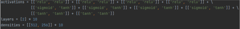
Figure 7: Snippet of NN code.
To train our Neural Network model, we used tensorflow to create our neural network model and sklearn to look at the accuracy and compute mean squared error for the loss. The activations we utilized are discussed below:
ReLU
We used ReLU as it is becoming increasingly popular in neural network models. It works well in avoiding the vanishing gradient, however, it struggles in representing models that contain many negatives. Here is a graph of the ReLU function:
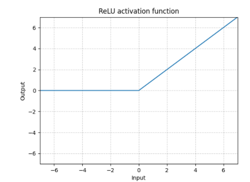
Figure 8: ReLU.
The reason ReLU avoids the vanishing gradient problem is due to its linear nature. Increasing greater values for the input only serves to output a linear increasing output, thus ensuring that the difference between two inputs is never essentially 0.
Sigmoid
Sigmoid is one of the most basic activation functions, but it is also useful. The strength of sigmoid is that input values that are further away from the center value have a much greater difference in output values, and thus in turn the function is better able to differentiate between smaller changes in data. However, this function fails to account for the vanishing gradient problem, shown below:
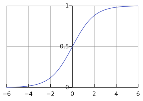
Figure 9: Sigmoid.
Tanh
We chose to use tanh for its more straightforward behavior in comparison to sigmoid:
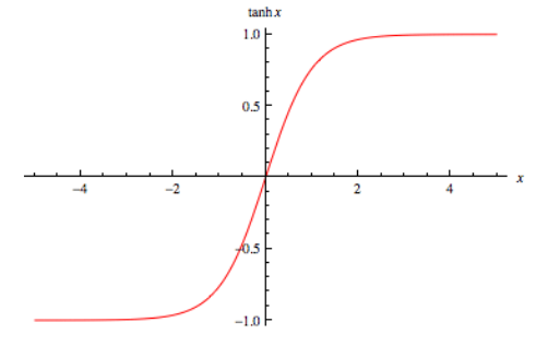
Figure 10: Tanh.
Like with the sigmoid function, this activation clearly doesn’t avoid the vanishing gradient problem. However, it’s more linear property around the middle is the relationship we tried to harness.
Unlike the other regression models, we were not able to directly implement cross validation. Instead, we manually split the data into train/test segments.
For brevity, we only discuss the best performing model in the Results section.
Results
Classification
To analyze the results of our classification model, we employed the use of confusion matrices, classification reports, and related metrics such as accuracy, precision, and recall. Unfortunately, we found that the Decision Tree classification model only gave us 2% accuracy along with a weighted F1-score of 2% and a weighted precision of only 1% in both data configurations tested, as can be observed in the images of the outputs below. Using all 19 features with the cleaned dataset compared to using the cleaned dataset with a reduced set of features gave almost the same suboptimal results. We believe this occurred because binning of the diameters removed key patterns that were necessary to properly identify diameters.
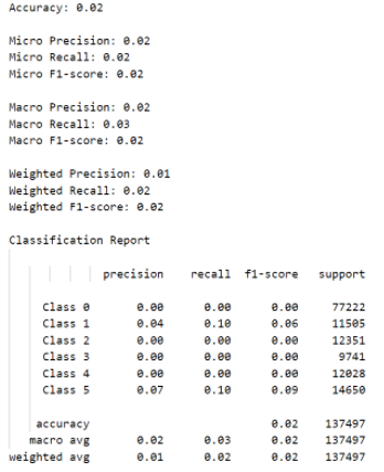
Figure 11: Metrics for Classification without PCA.
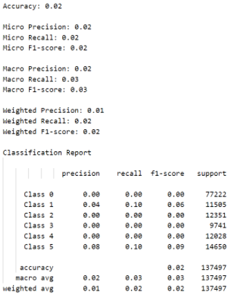
Figure 12: Metrics for Classification with PCA.
Regression
Ridge Regression
Utilizing the PCA reduced data with 3 dimensions gave us a minimum root mean squared error of 6.36 kilometers. As discussed previously, we found that asteroid features albedo and luminosity (H) are used frequently to approximate the size of an asteroid [12]. We reran Ridge regression on the reduced set of features and achieved a minimum root mean squared error of 5.68 kilometers which was only slightly better, representing a delta of 0.68 kilometers between the two approaches.
Lasso Regression
Utilizing the PCA reduced data with 3 dimensions gave us a minimum root mean squared error of 6.14 kilometers which, again, was surprisingly far from optimal, and constituted a very large error relative to the known diameter of asteroids. Utilizing only albedo and H resulted in a minimum root mean squared error of 5.32 kilometers, representing a delta of 0.82 kilometers between the two approaches.
Random Forest Regression
Using sklearn.ensemble.RandomForestRegressor on our original three features from PCA gave us a minimum root mean squared error of 4.42 kilometers. Rerunning the random forest regressor utilizing only albedo and luminosity once more resulted in significant improvement in our root mean squared error, bringing it to only 1.26 kilometers, representing a delta of 3.16 kilometers between the two approaches.
XGBoost Regressor
Experiments with the XGBoost regressor on the PCA-reduced dataset resulted in a minimum root mean squared error of 4.64 kilometers. Utilizing only albedo and luminosity, we were able to achieve a significantly better minimum root mean squared error of 1.26 kilometers, representing a delta of 3.38 kilometers between the two approaches.
Neural Network
We struggled to find a combination of activation functions, densities, and hyperparameters that would net us an root mean squared error value that was less than 0.972 kilometers. However, while we could not find further improvement, at this error level, the Neural Network performs significantly better than all other types of regressors we tested.
With only albedo and H as feature inputs, the best performing model achieved an average RMSE score of ~0.99. This model utilized ReLU activations for both layers, which had densities of 512, followed by 256 neurons. Below is the loss graph for train and test data at each epoch:
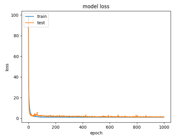
Figure 13: NN Loss graph with only albedo and H.
As we can see, the loss changes as expected for both the train and test data. After approximately epoch 100, we notice that the model converges, and any further reductions in loss are minimal.
With the other data input configuration using albedo, H, and per_y, the best performing model tested achieved an average root mean squared error score of ~0.972, once again utilizing ReLU activations for both hidden layers, and hidden layer densities of 512 followed by 256. Below is the loss graph for train and test data at each epoch:
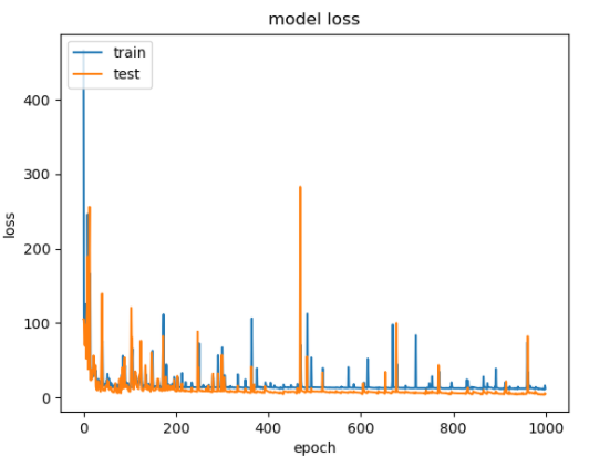
Figure 14: NN Loss graph with albedo, H, and per_y.
Interestingly, unlike in the other experiment included above, we notice spikes in the train and test loss. We believe these spikes occur due to outliers in the data, but were unable to derive any concrete conclusions why we observed this behavior in the results. Further, due to the instability in the graph, we don’t see the model converge until after epoch 200, at which point, excluding the spikes, the loss does not change significantly with additional training.
Discussion
We struggled to identify a combination of features that would be sufficiently separable for a regressor to learn. Initially, our exploration utilizing PCA on 19 selected features did not suffice to create a separable space in which the regressors could learn. Likewise, the covariance matrix for these features showed strong correlation between features that, given domain knowledge, are known to not be related to the diameter of an asteroid. As such, we conducted further feature engineering work to reduce the number of features down to two: Albedo and H (luminosity). As previously shown, Albedo does not have a strong correlation with diameter, but luminosity does.
Synthesizing the results from all of our experiments, we noticed a number of trends. First, we noticed that certain data performed very poorly relative to others. In particular, some data splits utilized during cross validation consistently resulted in a root mean squared error of 7.65 kilometers with the best hyperparameters for XGBoostRegressor, and 7.17 kilometers with the best hyperparameters for RandomForestRegressor. Given the aforementioned results about mean root squared error for both of those regressors, it’s clear that these data were in some ways outliers relative to the other data. Excluding this set of outlier data, we observe an average root mean squared error of 0.6 kilometers across the remainder of the data. Given that the median diameter of asteroids in the dataset is 3.95 kilometers (we don’t utilize mean here because outliers skew the mean significantly), this equates to an approximate error of 15%. Due to time constraints, we were unable to identify the root cause for why these outlier data points performed significantly worse than the rest of the data. We believe that future work could explore this phenomenon in more detail to get a better understanding of why certain asteroids do not follow the same trends.
As discussed earlier, we tested each regressor on two different sets of data. The first set had 19 PCA reduced features, and the second set used only albedo and H (luminosity). In each case, we can see that the overall performance of the regressor improved, with the delta ranging from 0.68 to 3.16. This corresponds to a 17% to 80% reduction in error. The improved performance in our regressors using the second feature set corresponded with existing properties known about asteroids [12].
Conclusions
Accurately predicting the diameter of an asteroid is a difficult task. Much of the feature data that is available for asteroids does not strongly correlate with their diameters. We explored a number of different algorithms, under different learning scenarios with different data, to determine if a potential accurate prediction model exists. Unfortunately, the best approximate error we were able to realize upon completing our experiments was on the order of 15% after outliers were removed.
Future work could include exploring a combination of supervised and unsupervised learning techniques to integrate the remaining data samples that were initially removed as a result of a lack of known diameter. Due to time and people constraints (we lost a team member early on in the semester), we were unable to explore this route. Additionally, generating new secondary features from the metadata regarding asteroids might potentially result in better diameter prediction. For instance, a domain expert could utilize their knowledge that a given type of asteroid has a specific type of composition, which in turn impacts the likelihood of that asteroid having a given diameter.
Additionally, spending more time investigating a neural network based approach, including exploring larger architectures with additional input features, might result in a much better regression model.
References
[1] https://www.sciencedirect.com/science/article/pii/S0019103504003811
[2] https://solarsystem.nasa.gov/asteroids-comets-and-meteors/asteroids/in-depth/
[3] https://arxiv.org/pdf/2007.05600.pdf
[4] https://www.kaggle.com/basu369victor/prediction-of-asteroid-diameter
[5] https://scikit-learn.org/stable/modules/generated/sklearn.manifold.TSNE.html
[6] https://scikit-learn.org/stable/modules/manifold.html#locally-linear-embedding
[7] https://scikit-learn.org/stable/modules/generated/sklearn.preprocessing.StandardScaler.html
[8] https://scikit-learn.org/stable/modules/generated/sklearn.linear_model.LinearRegression.html
[9] https://neptune.ai/blog/random-forest-regression-when-does-it-fail-and-why
[10] https://scikit-learn.org/stable/modules/generated/sklearn.ensemble.RandomForestRegressor.html
[11] https://medium.datadriveninvestor.com/random-forest-regression-9871bc9a25eb
[12] https://cneos.jpl.nasa.gov/tools/ast_size_est.html
[13] http://adsabs.harvard.edu/full/2007JBAA..117..342D
[14] https://scikit-learn.org/stable/modules/generated/sklearn.linear_model.Lasso.html
[15] https://scikit-learn.org/stable/modules/generated/sklearn.tree.DecisionTreeClassifier.html